An Introduction to Spatial Econometrics in R
This tutorial was prepared for the Ninth Annual Midwest Graduate Student Summit on Applied Economics, Regional, and Urban Studies (AERUS) on April 23rd-24th, 2016 at the University of Illinois at Urbana Champaign.
This notes illustrate the usage of R for spatial econometric analysis. The theory is heavily borrowed from Anselin and Bera (1998) and Arbia (2014) and the practical aspect is an updated version of Anselin (2003), with some additions in visualizing spatial data on R.
What’s R and why use it?
R is a free, open-source, and object oriented language. Free and open-source means that anyone is free to use, redistribute and change the software in any way. Moreover, “R is a free software environment for statistical computing and graphics. It compiles and runs on a wide variety of UNIX platforms, Windows and MacOS.” (http://cran.r-project.org)
There are lot of software out there to do data analysis that are prettier and seem easier than R, so why should I invest learning R? There are in my opinion at least three characteristics of R that make it worthwhile learning it. First of all, it is free. Many fancier looking software used today are quite expensive, but R is free and is going to be always free. R also is a language, which means that you don’t only get to use the functions that are build in the software but you can create your own (just to get an on the of the power of the R language you can take a look Professor Koenker’s Quantile Regression package). The last reason is that R is extremely well supported. If you have a question you just can Google it, post it to StackOverflow or use R-blogger. If you are not convinced yet, just can type “why use the R language”” in Google and I think the results will speak by themselves. All these characteristics plus the fact that researchers at the frontier of the profession use R as part of their research make R a great tool for spatial data analysis.
Introduction to spatial analysis in R
Motivation for using spatial analysis
Probably the most important argument for taking a spatial approach is that the independence assumption between observation is no longer valid. Attributes of observation i may influence the attributes of observation j.
To illustrate a very small set of what can be achieved in R for spatial analysis our running example will be examining violent crimes and foreclosures in the City of Chicago. The crime data as well as tracts shapefiles used here comes from Chicago Data Portal while foreclosures data come from the U.S. Department of Housing and Urban Development (HUD), all of these are public available.
R packages for spatial data analysis.
In R, the fundamental unit of shareable code is the package. A package bundles together code, data, documentation, and tests, and is easy to share with others. As of April 2016, there were over 8,200 packages available on the Comprehensive R Archive Network, or CRAN, the public clearing house for R packages. This huge variety of packages is one of the reasons that R is so successful: the chances are that someone has already solved a problem that you’re working on, and you can benefit from their work by downloading their package. (Wickham (2015))
Today we’ll focus on three packages maptools (R. Bivand and Lewin-Koh (2016)), spdep (R. Bivand and Piras (2015), R. Bivand, Hauke, and Kossowski (2013)) and leaflet (Cheng and Xie (2015)) and use a fourth one, the RColorBrewer package (Neuwirth (2014)) to make our plots more attractive. To install the packages, we simple have to type
install.packages("maptools", dependencies = TRUE)
install.packages("spdep", dependencies = TRUE)
install.packages("leaflet", dependencies = TRUE)
install.packages("RColorBrewer", dependencies = TRUE)
The maptools package has the functions needed to read geographic data, in particular ESRI shapefiles. The spdep package on the other hand contains the functions that will use in the spatial data analysis. The dependencies option installs uninstalled packages which these packages depend on. To access the functions and data in the package we must first call it. The function to call a package is library
library(spdep)
## Loading required package: sp

## Loading required package: Matrix
library(maptools)
## Checking rgeos availability: TRUE
Now that the packages are loaded we can read in our data.
Reading and Mapping spatial data in R
Spatial data comes in many “shapes” and “sizes”, the most common types of spatial data are:
- Points are the most basic form of spatial data. Denotes a single point location, such as cities, a GPS reading or any other discrete object defined in space.
- Lines are a set of ordered points, connected by straight line segments
- Polygons denote an area, and can be thought as a sequence of connected points, where the first point is the same as the last
- Grid (Raster) are a collection of points or rectangular cells, organized in a regular lattice
For more details, see R. S. Bivand, Pebesma, and Gomez-Rubio (2008). Today we’ll focus on Polygons. Spatial data usually comes in shapefile. This type of files stores non topological geometry and attribute information for the spatial features in a data set. Moreover, they don’t require a lot of disk space and are easy to read and write. (ESRI (1998))
First we have to download and save the files in our computer from our server at http://www.econ.uiuc.edu/~lab/workshop/foreclosures/. I saved mine in my desktop. We’ve downloaded 3 files:
- Main file: foreclosures.shp
- Index file: foreclosures.shx
- dBASE table: foreclosures.dbf
The main file describes a shape with a list of its vertices. In the index file, each record contains the offset of the corresponding main file record from the beginning of the main file. The dBASE table contains feature attributes with one record per feature. (ESRI (1998))
To read data from a polygon shapefile into R we use the function readShapePoly that will create a SpatialPolygonsDataFrame object. To learn more about the function, the command ?readShapePoly will give you access to the help file.
But before reading in the shapefile we first set our working directory. R is always pointing to a directory on your computer, to find which one use getwd() (get working directory). To specify a working directory:
setwd('~/Desktop/foreclosures')
On windows you may have to use \. The foreclosures folder contain the shapefiles that I downloaded before. Now we are ready to read in our shapefile.
chi.poly <- readShapePoly('foreclosures.shp')
the shapefile is now read and stored in an object called chi.poly. To check that it is a SpatialPolygonsDataFrame we can use the function class
class(chi.poly)
## [1] "SpatialPolygonsDataFrame"
## attr(,"package")
## [1] "sp"
A SpatialPolygonsDataFrame objects brings together the spatial representations of the polygons with data. The identifying tags of the polygons in the slot are matched with the row names of the data frame to make sure that the correct data rows are associated with the correct spatial object. (R. S. Bivand, Pebesma, and Gomez-Rubio (2008))
This object has four “parts” or slots: the first one is the data slot that contains the variables that will be used for our analysis; the second one is the polygon slot and contains the “shape” information. The third slot, bbox, is the bounding box drawn around the boundaries and the fourth slot is the proj4string which contains the projections. To access the data slot we can use the slot function or the @ symbol. For a compact look of the data slot we can use the str function:
str(slot(chi.poly,"data"))
## 'data.frame':    897 obs. of  16 variables:
##  $ SP_ID     : Factor w/ 897 levels "1","10","100",..: 1 112 223 334 445 556 667 778 887 2 ...
##  $ fips      : Factor w/ 897 levels "17031010100",..: 1 2 3 4 5 6 7 8 9 10 ...
##  $ est_fcs   : int  43 129 55 21 64 56 107 43 7 51 ...
##  $ est_mtgs  : int  904 2122 1151 574 1427 1241 1959 830 208 928 ...
##  $ est_fcs_rt: num  4.76 6.08 4.78 3.66 4.48 4.51 5.46 5.18 3.37 5.5 ...
##  $ res_addr  : int  2530 3947 3204 2306 5485 2994 3701 1694 443 1552 ...
##  $ est_90d_va: num  12.61 12.36 10.46 5.03 8.44 ...
##  $ bls_unemp : num  8.16 8.16 8.16 8.16 8.16 8.16 8.16 8.16 8.16 8.16 ...
##  $ county    : Factor w/ 1 level "Cook County": 1 1 1 1 1 1 1 1 1 1 ...
##  $ fips_num  : num  1.7e+10 1.7e+10 1.7e+10 1.7e+10 1.7e+10 ...
##  $ totpop    : int  5391 10706 6649 5325 10944 7178 10799 5403 1089 3634 ...
##  $ tothu     : int  2557 3981 3281 2464 5843 3136 3875 1768 453 1555 ...
##  $ huage     : int  61 53 56 60 54 58 48 57 61 48 ...
##  $ oomedval  : int  169900 147000 119800 151500 143600 145900 153400 170500 215900 114700 ...
##  $ property  : num  646 914 478 509 641 612 678 332 147 351 ...
##  $ violent   : num  433 421 235 159 240 266 272 146 78 84 ...
##  - attr(*, "data_types")= chr  "C" "C" "N" "N" ...
The first part is the data.frame part that contains the data for our analysis. We can see the variables contained in the data portion of the file including:
- est_fcs: estimated count of foreclosure starts from Jan. 2007 through June 2008
- est_mtgs: estimated number of active mortgages from Jan. 2007 through June 2008
- est_fcs_rt: number of foreclosure starts divided by number of mortgages times 100
- bls_unemp: June 2008 place or county unemployment rate
- totpop: total population from 2000 Census
- violent: number of violent crimes reported between Jan. 2007 through December 2008
- property: number of property crimes reported between Jan. 2007 through December 2008
We can also get summary statistics of the variables of interest using the function summary. For example,
summary(chi.poly@data$violent)
##    Min. 1st Qu.  Median    Mean 3rd Qu.    Max.
##     0.0    49.0   103.0   169.3   226.0  1521.0
Here we accessed the data portion of the shapefile with the @ sign and then the variable with the $ sign. To see the other slots, we can proceed in the same fashion.
A nice feature of the class of spatial objects is that we can use the traditional plotting features of R. The following command give’s us a plot of Chicago’s Census Tracts:
plot(chi.poly)
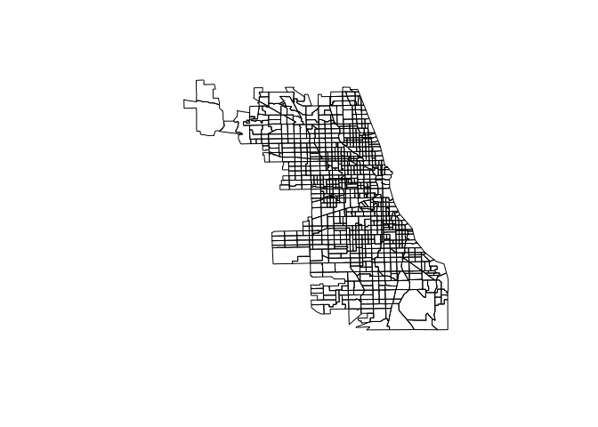
but we can go a step further and make nicer plots using the leaflet package. This generates an interactive map that can be rendered on HTML pages.
library(leaflet)
leaflet(chi.poly) %>%
  addPolygons(stroke = FALSE, fillOpacity = 0.5, smoothFactor = 0.5) %>%
  addTiles() #adds a map tile, the default is OpenStreetMap
we can add color using the package RColorBrewer
require(RColorBrewer)
## Loading required package: RColorBrewer
qpal<-colorQuantile("OrRd", chi.poly@data$violent, n=9) #define a palette with 7 breaks

leaflet(chi.poly) %>%
  addPolygons(stroke = FALSE, fillOpacity = .8, smoothFactor = 0.2, color = ~qpal(violent)
  ) %>%
  addTiles()
## Warning in doColorRamp(colorMatrix, x, alpha, ifelse(is.na(na.color), "", :
## '.Random.seed' is not an integer vector but of type 'NULL', so ignored
The colorQuantile function of the leaflet package maps values of the data to colors following a palette. In this case I’ve specified a palette of Oranges and Reds, for more palettes you can access the help file for RColorBrewer: ?RColorBrewer.
Spatial Econometrics in R
When dealing with space one must bear in mind Tobler’s first law of geography “Everything is related to everything else, but close things are more related than things that are far apart”(Tobler (1979)). In this section we’ll focus on the specification of spatial dependence, on specification tests to detect spatial dependence in regressions models and on basic regression models that incorporate spatial dependence. We’ll illustrate this using the data in the shapefile loaded in the previous section.
OLS
The traditional approach for many years has been to ignore the spatial dependence of the data and just run an OLS regression.
\[y = X \beta + \epsilon\]In R this is achieved with the lm function. For example,
chi.ols<-lm(violent~est_fcs_rt+bls_unemp, data=chi.poly@data)
I’ve specified the “model” as violent~est_fcs_rt+bls_unemp where violent is the dependent variable and, est_fcs_rt and bls_unemp are the explanatory variable. I’ve also specified the data set which is the slot data of our shapefile. Note that to access this slot I use the @ symbol. This line does not return anything because we have created an lm object that I called chi.ols. To see the results, we use the summary function
summary(chi.ols)
##
## Call:
## lm(formula = violent ~ est_fcs_rt + bls_unemp, data = chi.poly@data)
##
## Residuals:
##     Min      1Q  Median      3Q     Max
## -892.02  -77.02  -23.73   41.90 1238.22
##
## Coefficients:
##             Estimate Std. Error t value Pr(>|t|)
## (Intercept)  -18.627     45.366  -0.411    0.681
## est_fcs_rt    28.298      1.435  19.720   <2e-16 ***
## bls_unemp     -0.308      5.770  -0.053    0.957
## ---
## Signif. codes:  0 '***' 0.001 '**' 0.01 '*' 0.05 '.' 0.1 ' ' 1
##
## Residual standard error: 157.3 on 894 degrees of freedom
## Multiple R-squared:  0.3141, Adjusted R-squared:  0.3126
## F-statistic: 204.7 on 2 and 894 DF,  p-value: < 2.2e-16
The problem with ignoring the spatial structure of the data implies that the OLS estimates in the non spatial model may be biased, inconsistent or inefficient, depending on what is the true underlying dependence (for more see Anselin and Bera (1998)).
Modeling Spatial Dependence
We now take a closer look at spatial dependence, or to be more precise on it’s weaker expression spatial autocorrelation. Spatial autocorrelation measures the degree to which a phenomenon of interest is correlated to itself in space (Cliff and Ord (1973)). In other words, similar values appear close to each other, or cluster, in space (positive spatial autocorrelation) or neighboring values are dissimilar (negative spatial autocorrelation). Null spatial autocorrelation indicates that the spatial pattern is random. Following Anselin and Bera (1998) we can express the existence of spatial autocorrelation with the following moment condition:
\begin{equation} Cov(y_{i},y_{j})\neq 0\,\,\,\, for\,\,\,\,i\neq j \end{equation} were yi and yj are observations on a random variable at locations i and j. The problem here is that we need to estimate N by N covariance terms directly for N observations. To overcome this problem we impose restrictions on the nature of the interactions. One type of restriction is to define for each data point a relevant “neighborhood set”. In spatial econometrics this is operationalized via the spatial weights matrix. The matrix usually denoted by W is a N by N positive and symmetric matrix which denotes fore each observation (row) those locations (columns) that belong to its neighborhood set as nonzero elements (Anselin and Bera (1998), Arbia (2014)), the typical element is then:
\[\begin{equation} [w_{ij}]=\begin{cases} 1 & if\,j\in N\left(i\right) \\ 0 & o.w \end{cases} \end{equation}\]N(i) being the set of neighbors of location j. By convention, the diagonal elements are set to zero, i.e. \(w_{ii} = 0\). To help with the interpretation the matrix is often row standardized such that the elements of a given row add to one.
The specification of the neighboring set is quite arbitrary and there’s a wide range of suggestions in the literature. One popular way is to use one of the two following criteria:
- Rook criterion: two units are close to one another if they share a side
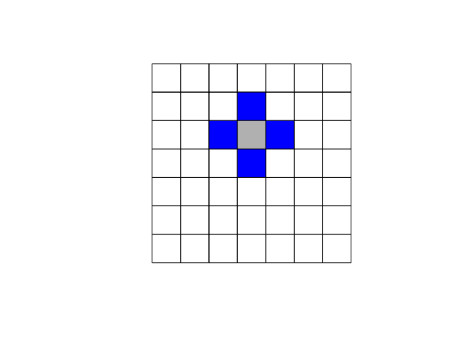
- Queen criterion: two units are close if they share a side or an edge.
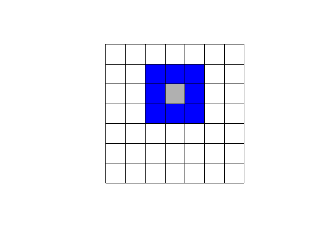
Another used approach is to denote two observations as neighbors if they are within a certain distance, i.e., \(j \in N(j) \ \ if d_{ij} \ < d_{max}\) where \(d\) is the distance between location \(i\) and \(j\) .
Here we’ll focus on using the queen criterion and we encourage the reader to experiment with the rook criterion. In R to obtain the weights matrix we make use of two functions. In the first step we use poly2nb which builds a neighbors list, if the option queen=TRUE is specified it will be build using the queen criterion. If FALSE is specified, then the rook criteria will be used. The next step is to supplement the neighbors list with the spatial weights. The option W row standardizes the matrix.
list.queen<-poly2nb(chi.poly, queen=TRUE)
W<-nb2listw(list.queen, style="W", zero.policy=TRUE)
W
## Characteristics of weights list object:
## Neighbour list object:
## Number of regions: 897
## Number of nonzero links: 6140
## Percentage nonzero weights: 0.7631036
## Average number of links: 6.845039
##
## Weights style: W
## Weights constants summary:
##     n     nn  S0       S1       S2
## W 897 804609 897 274.4893 3640.864
We can plot the link distribution with the usual plot function
plot(W,coordinates(chi.poly))
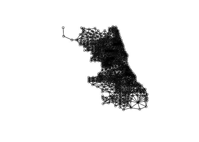
To obtain the weight matrix based on distances we use two functions: coordinates that will retrieve the centroid coordinates of the census tracts polygons and dnearneigh that will identify neighbors between two distances in kilometers measured using Euclidean distance. For example, to find neighbors within 1 kilometer we do:
coords<-coordinates(chi.poly)
W_dist<-dnearneigh(coords,0,1,longlat = FALSE)
I encourage you to compare the link distributions for these three ways of defining neighbors.
Spatial Autoregressive (SAR) Models
Spatial lag dependence in a regression setting can be modeled similar to an autoregressive process in time series. Formally,
\[y = \rho Wy + X \beta + \epsilon\]The presence of the term \(Wy\) induces a nonzero correlation with the error term, similar to the presence of an endogenous variable, but different from the time series context. Contrarious to time series, \([Wy]_i\) is always correlated with \(\epsilon\) irrespective of the structure of the errors. This implies that OLS estimates in the non spatial model will be biased and inconsistent. (Anselin and Bera (1998))
Spatial Error Models (SEM)
Another way to model spatial autocorrelation in a regression model is to specify the autoregressive process in the error term:
\[y = X \beta + \epsilon\]with
\[\epsilon = \lambda W \epsilon + u\]If this is the “true” form of spatial dependence OLS estimates will be unbiased but inefficient.
Testing for spatial autocorrelation
There are multiple tests for testing the presence of spatial autocorrelation. In this note we’ll focus on a restricted set: Moran’s I test and Lagrange Multiplier tests.
Moran’s I Test
Moran’s I test was originally developed as a two-dimensional analog of Durbin-Watson’s test
\[\begin{equation} I = \left( \frac{e'We}{e'e} \right) \end{equation}\]where \(e = y − X\beta\) is a vector of OLS residuals, \(\beta = (X'X)^{-1} X'y\), \(W\) is the row standardized spatial weights matrix.(For more detail see Anselin and Bera (1998))
To perform a Moran test on our data we need two inputs, an lm regression object (estimated in the OLS section) and the spatial weight matrix
moran.lm<-lm.morantest(chi.ols, W, alternative="two.sided")
print(moran.lm)
##
##  Global Moran I for regression residuals
##
## data:
## model: lm(formula = violent ~ est_fcs_rt + bls_unemp, data =
## chi.poly@data)
## weights: W
##
## Moran I statistic standard deviate = 11.785, p-value < 2.2e-16
## alternative hypothesis: two.sided
## sample estimates:
## Observed Moran I      Expectation         Variance
##     0.2142252370    -0.0020099108     0.0003366648
The computation of the statistic is relative to a given choice of the spatial weights W. Different specifications of the weights matrix will give different results. I encourage the reader to try this with the rook contiguity criterion.
Lagrange Multiplier Test
A nice feature of Moran’s I test is that i has high power against a wide range of alternatives (Anselin and Bera (1998)). However, it does not guide us in the selection of alternative models. On the other hand, Lagrange Multiplier test specify the alternative hypothesis which will help us with the task. The LM tests for spatial dependence are included in the lm.LMtests function and include as alternatives the presence of a spatial lag and the presence of a spatial lag in the error term. Both tests, as well as their robust forms are included in the lm.LMtests function. To call them we use the option test="all". Again, a regression object and a spatial listw object must be passed as arguments:
LM<-lm.LMtests(chi.ols, W, test="all")
print(LM)
##
##  Lagrange multiplier diagnostics for spatial dependence
##
## data:
## model: lm(formula = violent ~ est_fcs_rt + bls_unemp, data =
## chi.poly@data)
## weights: W
##
## LMerr = 134.52, df = 1, p-value < 2.2e-16
##
##
##  Lagrange multiplier diagnostics for spatial dependence
##
## data:
## model: lm(formula = violent ~ est_fcs_rt + bls_unemp, data =
## chi.poly@data)
## weights: W
##
## LMlag = 182.18, df = 1, p-value < 2.2e-16
##
##
##  Lagrange multiplier diagnostics for spatial dependence
##
## data:
## model: lm(formula = violent ~ est_fcs_rt + bls_unemp, data =
## chi.poly@data)
## weights: W
##
## RLMerr = 0.00066762, df = 1, p-value = 0.9794
##
##
##  Lagrange multiplier diagnostics for spatial dependence
##
## data:
## model: lm(formula = violent ~ est_fcs_rt + bls_unemp, data =
## chi.poly@data)
## weights: W
##
## RLMlag = 47.653, df = 1, p-value = 5.089e-12
##
##
##  Lagrange multiplier diagnostics for spatial dependence
##
## data:
## model: lm(formula = violent ~ est_fcs_rt + bls_unemp, data =
## chi.poly@data)
## weights: W
##
## SARMA = 182.18, df = 2, p-value < 2.2e-16
Since LMerr and LMlag are both statistically significant different from zero, we need to look at their robust counterparts. These robust counterparts are actually robust to the presence of the other “type” of autocorrelation. The robust version of the tests suggest that the lag model is the more likely alternative.
Running Spatial Regressions
SAR Models
The estimation of the SAR model can be approached in two ways. One way is to assume normality of the error term and use maximum likelihood. This is achieved in R with the function lagsarlm
sar.chi<-lagsarlm(violent~est_fcs_rt+bls_unemp, data=chi.poly@data, W)
summary(sar.chi)
##
## Call:
## lagsarlm(formula = violent ~ est_fcs_rt + bls_unemp, data = chi.poly@data,
##     listw = W)
##
## Residuals:
##      Min       1Q   Median       3Q      Max
## -519.127  -65.003  -15.226   36.423 1184.193
##
## Type: lag
## Coefficients: (asymptotic standard errors)
##             Estimate Std. Error z value Pr(>|z|)
## (Intercept) -93.7885    41.3162  -2.270  0.02321
## est_fcs_rt   15.6822     1.5600  10.053  < 2e-16
## bls_unemp     8.8949     5.2447   1.696  0.08989
##
## Rho: 0.49037, LR test value: 141.33, p-value: < 2.22e-16
## Asymptotic standard error: 0.039524
##     z-value: 12.407, p-value: < 2.22e-16
## Wald statistic: 153.93, p-value: < 2.22e-16
##
## Log likelihood: -5738.047 for lag model
## ML residual variance (sigma squared): 20200, (sigma: 142.13)
## Number of observations: 897
## Number of parameters estimated: 5
## AIC: 11486, (AIC for lm: 11625)
## LM test for residual autocorrelation
## test value: 8.1464, p-value: 0.0043146
Another way is to use 2SLS using the function stsls. I leave this to the reader so he/she can compare the results to the MLE approach. The function is:
sar2sls.chi<-stsls(violent~est_fcs_rt+bls_unemp, data=chi.poly@data, W)
summary(sar2sls.chi)
We then can compare the residuals of the OLS regression to the residuals of the spatial autoregressive model. To access the residuals for the OLS model and the SAR model we simply do
chi.poly@data$chi.ols.res<-resid(chi.ols) #residuals ols

chi.poly@data$chi.sar.res<-resid(sar.chi) #residual sar
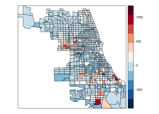
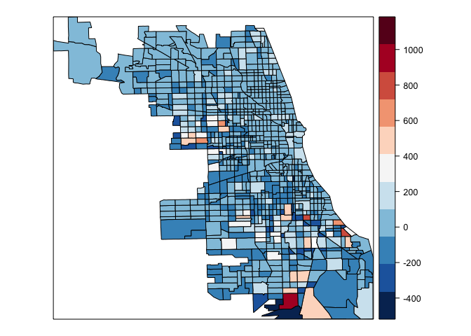
In this step I’ve create a new variable in the data portion of the shapefile that will help with the plotting of the residuals. To plot the residuals, I use the spplot function in the spdep package. The arguments are the shapefile, the variable that we want to plot, the number of breaks and the colors we are going to use. To specify the colors, we use the Red and Blues (RdBu) palette from the RColorBrewer package.
spplot(chi.poly,"chi.ols.res", at=seq(min(chi.poly@data$chi.ols.res,na.rm=TRUE),max(chi.poly@data$chi.ols.res,na.rm=TRUE),length=12),col.regions=rev(brewer.pal(11,"RdBu")))
spplot(chi.poly,"chi.sar.res",at=seq(min(chi.poly@data$chi.sar.res,na.rm=TRUE),max(chi.poly@data$chi.sar,na.rm=TRUE), length=12), col.regions=rev(brewer.pal(11,"RdBu")))
Marginal Effects
Note that the presence of the spatial weights matrix makes marginal effects richer and slightly more complicated than in the “traditional” OLS model. We’ll have three impact measures suggested by Pace and LeSage (2009) and is done in R with the function impacts
impacts(sar.chi, listw=W)
## Impact measures (lag, exact):
##               Direct  Indirect    Total
## est_fcs_rt 16.434479 14.336896 30.77137
## bls_unemp   9.321585  8.131842 17.45343
The direct impact refers to average total impact of a change of an independent variable on the dependent fore each observation, i.e., $n^{-1}\sum_{i=1}^{n}\frac{\partial E(y_{i})}{\partial X_{i}}$, the indirect impact which is the sum of the impact produced on one single observation by all other observations and the impact of one observation on all the other. The total is the summation of the two
SEM Models
On the other hand, if we want to estimate the Spatial Error Model we have two approaches again. First, we can use Maximum Likelihood as before, with the function errorsarlm
errorsalm.chi<-errorsarlm(violent~est_fcs_rt+bls_unemp, data=chi.poly@data, W)
summary(errorsalm.chi)
##
## Call:
## errorsarlm(formula = violent ~ est_fcs_rt + bls_unemp, data = chi.poly@data,
##     listw = W)
##
## Residuals:
##      Min       1Q   Median       3Q      Max
## -650.506  -64.355  -22.646   35.461 1206.346
##
## Type: error
## Coefficients: (asymptotic standard errors)
##             Estimate Std. Error z value Pr(>|z|)
## (Intercept)  -1.2624    43.0509 -0.0293   0.9766
## est_fcs_rt   19.4620     1.9450 10.0062   <2e-16
## bls_unemp     4.0380     5.5134  0.7324   0.4639
##
## Lambda: 0.52056, LR test value: 109.68, p-value: < 2.22e-16
## Asymptotic standard error: 0.042291
##     z-value: 12.309, p-value: < 2.22e-16
## Wald statistic: 151.51, p-value: < 2.22e-16
##
## Log likelihood: -5753.875 for error model
## ML residual variance (sigma squared): 20796, (sigma: 144.21)
## Number of observations: 897
## Number of parameters estimated: 5
## AIC: 11518, (AIC for lm: 11625)
The same plot for the SEM residuals can be done as before and is left for the reader. A second approach is use Feasible Generalized Least Squares (GLS) with the function GMerrorsar. The function is:
fgls.chi<-GMerrorsar(violent~est_fcs_rt+bls_unemp, data=chi.poly@data, W)
summary(fgls.chi)
Finally, if we look at the likelihood for the SAR model and SEM model we see that we achieve a lower value for the SAR model that was the model favored by the LMtests. The residuals plot presented above still show some presence of spatial autocorrelation. It’s very likely that the a more complete model is specified. The literature has expanded to more complex models. The reader is encouraged to read Anselin and Bera (1998), Arbia (2014) and Pace and LeSage (2009) for more detailed and complete introductions on Spatial Econometrics.
Comments and suggestions are always welcomed. You can send them to srmntbr2 at illinois.edu. The usual disclaimers apply.
References
Anselin, Luc. 2003. “An Introduction to Spatial Regression Analysis in R.” Available at: Https://Geodacenter.asu.edu/Drupal_files/Spdepintro.pdf.
Anselin, Luc, and Anil K Bera. 1998. “Spatial Dependence in Linear Regression Models with an Introduction to Spatial Econometrics.” Statistics Textbooks and Monographs 155. MARCEL DEKKER AG: 237–90.
Arbia, Giuseppe. 2014. A Primer for Spatial Econometrics: With Applications in R. Palgrave Macmillan.
Bivand, Roger S, Edzer J Pebesma, and Virgilio Gomez-Rubio. 2008. Applied Spatial Data Analysis with R. Springer. Springer.
Bivand, Roger, and Nicholas Lewin-Koh. 2016. Maptools: Tools for Reading and Handling Spatial Objects. https://CRAN.R-project.org/package=maptools.
Bivand, Roger, and Gianfranco Piras. 2015. “Comparing Implementations of Estimation Methods for Spatial Econometrics.” Journal of Statistical Software 63 (18): 1–36. http://www.jstatsoft.org/v63/i18/.
Bivand, Roger, Jan Hauke, and Tomasz Kossowski. 2013. “Computing the Jacobian in Gaussian Spatial Autoregressive Models: An Illustrated Comparison of Available Methods.” Geographical Analysis 45 (2): 150–79. http://www.jstatsoft.org/v63/i18/.
Cheng, Joe, and Yihui Xie. 2015. Leaflet: Create Interactive Web Maps with the Javascript ’Leaflet’ Library. http://rstudio.github.io/leaflet/.
Cliff, Andrew David, and J Keith Ord. 1973. Spatial Autocorrelation. Vol. 5. Pion London.
ESRI, Environmental Systems Research Institute. 1998. “ESRI Shapefile Technical Description.” Available at: Https://Www.esri.com/Library/Whitepapers/Pdfs/Shapefile.pdf.
Neuwirth, Erich. 2014. RColorBrewer: ColorBrewer Palettes. https://CRAN.R-project.org/package=RColorBrewer.
Pace, R Kelley, and JP LeSage. 2009. “Introduction to Spatial Econometrics.” Boca Raton, FL: Chapman &Hall/CRC.
Tobler, WR. 1979. “Cellular Geography.” In Philosophy in Geography, 379–86. Springer.
Wickham, Hadley. 2015. R Packages. “O’Reilly Media, Inc.”
Ignacio
Sarmiento Barbieri
University of Los Andes
- srmntbr2 (at) illinois.edu
- ignaciomsarmiento (at) gmail.com
- ignaciomsarmiento
Blogs/Links
These are blogs/sites I frequently visit