Lecture 1: Spatial Data

class: center, middle

#  Point Process Analysis

### Ignacio Sarmiento-Barbieri

---
# Tipos de Datos Espaciales

Los datos espaciales vienen en muchas "formas" y "tamaños", los tipos más comunes de datos espaciales son:

- **Punto**

- **Líneas**

- **Polígonos**

- **Grillas (*o raster*)**

---
# The earth ain't flat

---
# Projections

-  Geographic coordinate systems: coordinate systems that span the entire globe (e.g. latitude / longitude).
  
  - Projected coordinate systems: coordinate systems that are localized to minimize visual distortion in a particular region (e.g. Robinson, UTM, State Plane)
  
---
# Projections

<img src="figures/proj.png" width="800" style="display: block; margin: auto;" />
---
# Which projection should I choose?
- “There exist no all-purpose projections, all involve distortion when far from the center of the specified frame” (Bivand, Pebesma, and Gómez-Rubio 2013)
  
  - In some cases, it is not something that we are free to decide: “often the choice of projection is made by a public mapping agency” (Bivand, Pebesma, and Gómez-Rubio 2013).

-  This means that when working with local data sources, it is likely preferable to work with the CRS in which the data was provided.

- For Bogotá the IGAC promotes the adoption of MAGNA-SIRGAS. EPSG code: 4626

---
## Reading Spatial Data in R

Packages:

```r
require("sf")
```

```
## Loading required package: sf
```

```
## Linking to GEOS 3.10.2, GDAL 3.4.2, PROJ 8.2.1; sf_use_s2() is TRUE
```

```r
require("tidyverse")
require("here")
```

```
## Loading required package: here
```

```
## here() starts at /Users/ignaciosarmiento/Dropbox/Teaching/2022/SpatialDataEng/Lectures/Lecture2
```

---
## Reading Spatial Data in R

```r
bars<-st_read(here("egba/EGBa.shp"))
```

```
## Reading layer `EGBa' from data source 
##   `/Users/ignaciosarmiento/Dropbox/Teaching/2022/SpatialDataEng/Lectures/Lecture2/egba/EGBa.shp' 
##   using driver `ESRI Shapefile'
## Simple feature collection with 515 features and 7 fields
## Geometry type: POINT
## Dimension:     XY
## Bounding box:  xmin: -74.17607 ymin: 4.577897 xmax: -74.02929 ymax: 4.806253
## Geodetic CRS:  MAGNA-SIRGAS
```
---
## Visualizing Points

.pull-left[

```r
ggplot()+
  geom_sf(data=bars) +
  theme_bw() +
  theme(axis.title =element_blank(),
        panel.grid.major = element_blank(),
        panel.grid.minor = element_blank(),
        axis.text = element_text(size=6))
```
]

.pull-right[
![](Lecture2_files/figure-html/plot_bars-1.png)
]

---
class: center, middle

#  Point Process Methods
---
#  Questions

- Are the points spread uniformly over the survey region?

- Are the points randomly scattered?

- Is there evidence of clustering?

- Does the density of points depend on an explanatory variable?

To give a sensible answer we must recognise that these questions are not about the points themselves, but about the way the points were generated.
---

<img src="figures/point_realizations.png" width="900" height="600" style="display: block; margin: auto;" />
---
# Point Process and Notation

---
# Complete spatial randomness (CSR)

Properties:

- homogeneity

- independence

---
# CSR: homogeneity

---
# CSR: independence

---
# Simulation of CSR

```r
require("spatstat")
```

```
## Loading required package: spatstat
```

```
## Loading required package: spatstat.data
```

```
## Loading required package: spatstat.geom
```

```
## spatstat.geom 2.4-0
```

```
## 
## Attaching package: 'spatstat.geom'
```

```
## The following object is masked from 'package:scales':
## 
##     rescale
```

```
## Loading required package: spatstat.random
```

```
## spatstat.random 2.2-0
```

```
## Loading required package: spatstat.core
```

```
## Loading required package: nlme
```

```
## 
## Attaching package: 'nlme'
```

```
## The following object is masked from 'package:dplyr':
## 
##     collapse
```

```
## Loading required package: rpart
```

```
## spatstat.core 2.4-4
```

```
## Loading required package: spatstat.linnet
```

```
## spatstat.linnet 2.3-2
```

```
## 
## spatstat 2.3-4       (nickname: 'Watch this space') 
## For an introduction to spatstat, type 'beginner'
```

---
class: center
# Simulation of CSR

```r
set.seed(10101)
plot(rpoispp(50))
```

![](Lecture2_files/figure-html/unnamed-chunk-10-1.png)

---
class: center
# Simulation of CSR

```r
plot(rpoispp(100,nsim=6))
```

![](Lecture2_files/figure-html/unnamed-chunk-11-1.png)
---
# Inhomogeneous Poisson process

.pull-left[

```r
lambda <- function(x,y) { 100 * (x^2+y) } 
X <- rpoispp(lambda, win=square(1))
```
]
.pull-right[

```r
plot(X)
```

![](Lecture2_files/figure-html/unnamed-chunk-13-1.png)
]
---

class: center, middle

#  Exploratory Data Analysis
---
# Intensity

```r
plot(swedishpines, main = "")
```

![](Lecture2_files/figure-html/unnamed-chunk-14-1.png)
---
# Intensity

```r
npoints(swedishpines)/area(Window(swedishpines))
```

```
## [1] 0.007395833
```

```r
intensity(swedishpines)
```

```
## [1] 0.007395833
```

```r
unitname(swedishpines)
```

```
## 0.1 metres
```

---
# Estimating Homogeneous Intensity

```r
summary(swedishpines)
```

```
## Planar point pattern:  71 points
## Average intensity 0.007395833 points per square unit (one unit = 0.1 metres)
## 
## Coordinates are integers
## i.e. rounded to the nearest unit (one unit = 0.1 metres)
## 
## Window: rectangle = [0, 96] x [0, 100] units
## Window area = 9600 square units
## Unit of length: 0.1 metres
```

---
# Estimating Homogeneous Intensity

```r
intensity(rescale(swedishpines))
```

```
## [1] 0.7395833
```

---
# Estimating Homogeneous Intensity

```r
X <- rescale(swedishpines)
lam <- intensity(X)
(sdX <- sqrt(lam/area(Window(X))))
```

```
## [1] 0.08777239
```

---
# Quadrant Counting

```r
swp <- rescale(swedishpines)
Q3 <- quadratcount(swp, nx=3, ny=3)
Q3
```

```
##              x
## y             [0,3.2) [3.2,6.4) [6.4,9.6]
##   [6.67,10]         8         6         7
##   [3.33,6.67)       8        11         9
##   [0,3.33)          5         6        11
```

---
# Quadrant Counting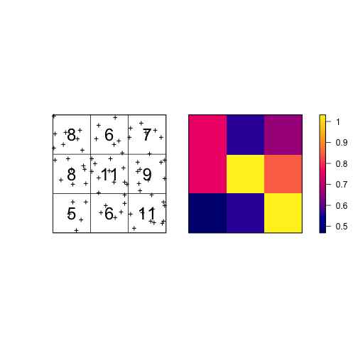

![](Lecture2_files/figure-html/unnamed-chunk-22-1.png)

---
# Quadrant Counting test for homogeneity

```r
intensity(Q3)
```

```
##              x
## y             [0,3.2) [3.2,6.4) [6.4,9.6]
##   [6.67,10]   0.75000   0.56250   0.65625
##   [3.33,6.67) 0.75000   1.03125   0.84375
##   [0,3.33)    0.46875   0.56250   1.03125
```

---
# Quadrant Counting test for homogeneity

```r
tS <- quadrat.test(swp, 3,3)
tS
```

```
## 
## 	Chi-squared test of CSR using quadrat counts
## 
## data:  swp
## X2 = 4.6761, df = 8, p-value = 0.4169
## alternative hypothesis: two.sided
## 
## Quadrats: 3 by 3 grid of tiles
```

```r
tS$p.value
```

```
## [1] 0.4168565
```

---
# Quadrant Counting test for homogeneity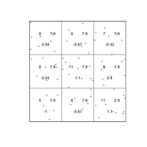
![](Lecture2_files/figure-html/unnamed-chunk-26-1.png)

---
# KDE

Sean `$(x_1, x_2, \cdots, x_n) \sim iid$` from some unknown `$f$`, we want to estimate it

`$$\hat{f_h}(x)=\frac{1}{nh}\sum_{i=1}^nK\left(\frac{x-x_i}{h}\right)$$`

---
# KDE
<img src="figures/fig1.png" width="500" height="400" style="display: block; margin: auto;" />

---
# KDE  Bandwidth

`\begin{align}
  MSE (\hat{f}(x)) = \left( Sesgo (\hat{f}(x))\right)^2 + Var (\hat{f}(x)) 
\end{align}`

La expresión aproximada en `$x_o$` está dada por

`\begin{align}
  Sesgo [\hat{f} (x_o)] \approx \frac{h^2}{2}  f''(x_o ) \int_{-\infty}^\infty K(\phi) \phi^2  d\phi   
\end{align}`

`\begin{align}
   Var [\hat{f} (x_o)] \approx \frac{1}{n\times h}  f(x_o ) \int_{-\infty}^\infty K^2(\phi)   d\phi   
\end{align}`

---
# KDE
<img src="figures/fig2.png" width="500" height="400" style="display: block; margin: auto;" />

---
# KDE
<img src="figures/fig3.png" width="500" height="400" style="display: block; margin: auto;" />

---
# KDE  Bandwidth

- Scott's Rule: `$h \approx 1.06⋅\hat{\sigma} n^{−1/5}$`.

- Silverman: `$h \approx 0.9 min \left\{\hat{\sigma}, \frac{IQR}{1.35}\right\} n^{−1/5}$`. 
   
   - Cross-Validation:

`\begin{align}
CV_k(h) = \frac{1}{n} \sum_{i=1}^n \log \hat{f}_{-k}(X_k)
\end{align}`

---
# KDE
<img src="figures/fig4.png" width="500" height="400" style="display: block; margin: auto;" />

---
### KDE: Kernel

Properties

1.  `$K(u)=K(-u)$`

2.  `$\int_{-\infty}^\infty K(u) du = 1$`

3. `$K'(u)<0$` when `$u>0$`

4. `$E[K]=0$`

---
### KDE: Kernel

<img src="figures/fig5.png" width="500" height="400" style="display: block; margin: auto;" />
---
### KDE: Kernel

---
### KDE: Kernel

---
### KDE: Kernel

---
### KDE: Kernel

Kernel functions:

- Gaussian 
  
  - Epanechnikov
  
  - Rectangular
  
  - Triangular

---
### KDE: Kernel

<img src="figures/fig9.png" width="500" height="400" style="display: block; margin: auto;" />
---
### KDE: Kernel

```r
db<-data.frame(place=c("CBD"),lat=c(4.651887), long=c(-74.05812))
db<-st_as_sf(db,coords=c('long','lat'),crs=4326) #EPSG:4326 - WGS 84, latitude/longitude coordinate system 
db<-st_transform(db, 4686)
z<-st_distance(bars,db)
head(z)
```

```
## Units: [m]
##          [,1]
## [1,] 4330.199
## [2,] 4330.199
## [3,] 4289.943
## [4,] 4372.001
## [5,] 4291.624
## [6,] 4403.613
```

---
### KDE: Kernel

```r
z<-units::set_units(z,"km")
head(z)
```

```
## Units: [km]
##          [,1]
## [1,] 4.330199
## [2,] 4.330199
## [3,] 4.289943
## [4,] 4.372001
## [5,] 4.291624
## [6,] 4.403613
```

---
### KDE: Kernel

```r
plot(density(z))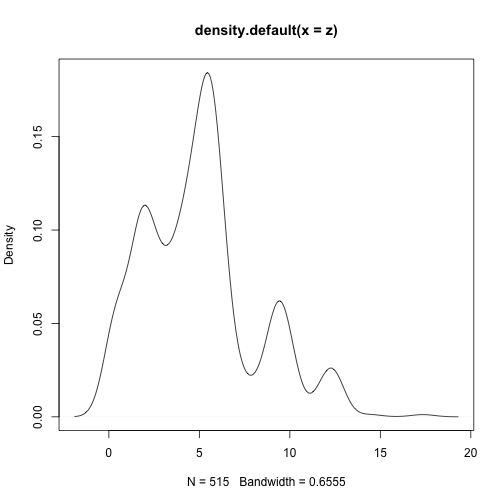
```

![](Lecture2_files/figure-html/unnamed-chunk-38-1.png)

---
### KDE: Kernel

```r
plot(density(z,bw="nrd0", kernel='gaussian'))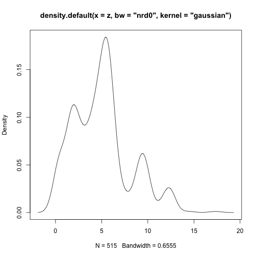
```

![](Lecture2_files/figure-html/unnamed-chunk-39-1.png)

---
### KDE: Kernel

```r
plot(density(z,bw="nrd0", kernel='epanechnikov'))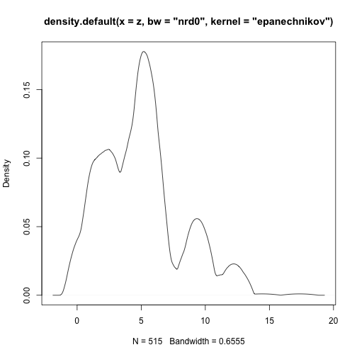
```

![](Lecture2_files/figure-html/unnamed-chunk-40-1.png)

---
### KDE: Kernel

```r
plot(density(z,bw="nrd0", kernel='rectangular'))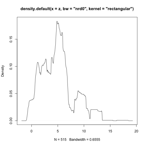
```

![](Lecture2_files/figure-html/unnamed-chunk-41-1.png)

---
### Bivariate KDE

`\begin{align}
\hat{f}(x;H):=\frac{1}{n|H|^{1/2}}\sum_{i=1}^nK\left(H^{-1/2}(\mathbf{x}-\mathbf{x}_i)\right)
\end{align}`

`\begin{align}
    \hat{f}(x,y) = \frac{1}{nh_xh_y}\sum_{i=1}^n K\left(\frac{X_i-x}{h_x}\right)K\left(\frac{Y_i-x}{h_y}\right)
\end{align}`

---
### Bivariate KDE

.pull-left[

```r
ggplot(bars, aes( x=LONGITUD, y=LATITUD) ) +
  geom_density_2d(size = 0.25, colour = "black") +
  theme_bw()
```
]

.pull-right[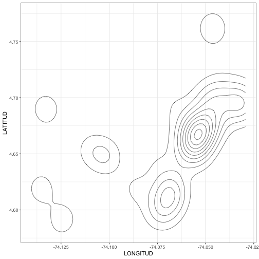
![](Lecture2_files/figure-html/plot-label3-out-1.png)
]

---
### Bivariate KDE

```r
require("SpatialKDE")

bars<-st_transform(bars,21818)

cell_size <- 2000
band_width <- 1000

grid_bars <- bars %>% 
  create_grid_rectangular(cell_size = cell_size, side_offset = band_width)
```

---
### Bivariate KDE

```r
kde <- bars %>% 
  kde(band_width = band_width, kernel = "epanechnikov", grid = grid_bars)
kde
```

```
## Simple feature collection with 100 features and 1 field
## Geometry type: POLYGON
## Dimension:     XY
## Bounding box:  xmin: 590396.2 ymin: 505070.2 xmax: 610396.2 ymax: 533070.2
## Projected CRS: Bogota 1975 / UTM zone 18N
## First 10 features:
##                          geometry kde_value
## 1  POLYGON ((590396.2 505070.2... 0.0000000
## 2  POLYGON ((592396.2 505070.2... 0.0000000
## 3  POLYGON ((594396.2 505070.2... 0.0000000
## 4  POLYGON ((596396.2 505070.2... 0.2990913
## 5  POLYGON ((598396.2 505070.2... 0.0000000
## 6  POLYGON ((600396.2 505070.2... 0.0000000
## 7  POLYGON ((602396.2 505070.2... 0.0000000
## 8  POLYGON ((590396.2 507070.2... 0.9865835
## 9  POLYGON ((592396.2 507070.2... 0.0000000
## 10 POLYGON ((594396.2 507070.2... 0.0000000
```
---
### Bivariate KDE

.pull-left[

```r
require("tmap")

tm_shape(kde) + 
  tm_polygons(col = "kde_value", palette = "viridis", title = "KDE Estimate") +
  tm_shape(bars) +
  tm_bubbles(size = 0.1, col = "red")
```
]

.pull-right[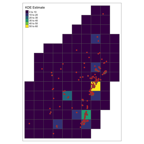
![](Lecture2_files/figure-html/plot-label-out-1.png)
]

---

```r
sessionInfo()
```

```
## R version 4.2.0 (2022-04-22)
## Platform: x86_64-apple-darwin17.0 (64-bit)
## Running under: macOS Big Sur/Monterey 10.16
## 
## Matrix products: default
## BLAS:   /Library/Frameworks/R.framework/Versions/4.2/Resources/lib/libRblas.0.dylib
## LAPACK: /Library/Frameworks/R.framework/Versions/4.2/Resources/lib/libRlapack.dylib
## 
## locale:
## [1] en_US.UTF-8/en_US.UTF-8/en_US.UTF-8/C/en_US.UTF-8/en_US.UTF-8
## 
## attached base packages:
## [1] stats     graphics  grDevices utils     datasets  methods   base     
## 
## other attached packages:
##  [1] tmap_3.3-3            SpatialKDE_0.7.0      spatstat_2.3-4       
##  [4] spatstat.linnet_2.3-2 spatstat.core_2.4-4   rpart_4.1.16         
##  [7] nlme_3.1-157          spatstat.random_2.2-0 spatstat.geom_2.4-0  
## [10] spatstat.data_2.2-0   here_1.0.1            sf_1.0-7             
## [13] scales_1.2.0          plotly_4.10.0         lubridate_1.8.0      
## [16] kableExtra_1.3.4      nomnoml_0.2.5         knitr_1.39           
## [19] forcats_0.5.1         stringr_1.4.0         dplyr_1.0.9          
## [22] purrr_0.3.4           readr_2.1.2           tidyr_1.2.0          
## [25] tibble_3.1.7          ggplot2_3.3.6         tidyverse_1.3.1      
## [28] xaringanExtra_0.5.5   xaringanthemer_0.4.1 
## 
## loaded via a namespace (and not attached):
##   [1] leafem_0.2.0          colorspace_2.0-3      deldir_1.0-6         
##   [4] ellipsis_0.3.2        class_7.3-20          leaflet_2.1.1        
##   [7] rprojroot_2.0.3       base64enc_0.1-3       fs_1.5.2             
##  [10] dichromat_2.0-0.1     rstudioapi_0.13       proxy_0.4-26         
##  [13] farver_2.1.0          xaringan_0.24         fansi_1.0.3          
##  [16] xml2_1.3.3            splines_4.2.0         codetools_0.2-18     
##  [19] polyclip_1.10-0       jsonlite_1.8.0        tmaptools_3.1-1      
##  [22] broom_0.8.0           dbplyr_2.1.1          png_0.1-7            
##  [25] spatstat.sparse_2.1-1 compiler_4.2.0        httr_1.4.3           
##  [28] backports_1.4.1       assertthat_0.2.1      Matrix_1.4-1         
##  [31] fastmap_1.1.0         lazyeval_0.2.2        cli_3.3.0            
##  [34] s2_1.0.7              htmltools_0.5.2       tools_4.2.0          
##  [37] gtable_0.3.0          glue_1.6.2            wk_0.6.0             
##  [40] Rcpp_1.0.8.3          raster_3.5-15         cellranger_1.1.0     
##  [43] jquerylib_0.1.4       vctrs_0.4.1           svglite_2.1.0        
##  [46] leafsync_0.1.0        crosstalk_1.2.0       lwgeom_0.2-8         
##  [49] xfun_0.30             rvest_1.0.2           lifecycle_1.0.1      
##  [52] XML_3.99-0.10         goftest_1.2-3         terra_1.5-21         
##  [55] MASS_7.3-56           hms_1.1.1             spatstat.utils_2.3-1 
##  [58] parallel_4.2.0        RColorBrewer_1.1-3    yaml_2.3.5           
##  [61] sass_0.4.1            stringi_1.7.6         highr_0.9            
##  [64] e1071_1.7-9           rlang_1.0.2           pkgconfig_2.0.3      
##  [67] systemfonts_1.0.4     evaluate_0.15         lattice_0.20-45      
##  [70] tensor_1.5            labeling_0.4.2        htmlwidgets_1.5.4    
##  [73] tidyselect_1.1.2      magrittr_2.0.3        R6_2.5.1             
##  [76] generics_0.1.2        DBI_1.1.2             pillar_1.7.0         
##  [79] haven_2.5.0           whisker_0.4           withr_2.5.0          
##  [82] mgcv_1.8-40           stars_0.5-5           units_0.8-0          
##  [85] sp_1.4-7              abind_1.4-5           modelr_0.1.8         
##  [88] crayon_1.5.1          KernSmooth_2.23-20    utf8_1.2.2           
##  [91] tzdb_0.3.0            rmarkdown_2.14        isoband_0.2.5        
##  [94] grid_4.2.0            readxl_1.4.0          data.table_1.14.2    
##  [97] reprex_2.0.1          digest_0.6.29         classInt_0.4-3       
## [100] webshot_0.5.3         munsell_0.5.0         viridisLite_0.4.0    
## [103] bslib_0.3.1
```